how-a-relational-database-works(原文)

原文出处 http://coding-geek.com/how-databases-work/

网上流传的翻译版看起来不错，费尽心思找到英文原版出处，看起来网站有了一定年头了，这里边读边做个记录保存，防止以后文章丢失。

这是一篇2015年发布的文章，对关系型数据库的整个工作流程介绍得比较清楚。

Preface

When it comes to relational databases, I can’t help thinking that something is missing. They’re used everywhere. There are many different databases: from the small and useful SQLite to the powerful Teradata. But, there are only a few articles that explain how a database works. You can google by yourself “how does a relational database work” to see how few results there are. Moreover, those articles are short. Now, if you look for the last trendy technologies (Big Data, NoSQL or JavaScript), you’ll find more in-depth articles explaining how they work.

Are relational databases too old and too boring to be explained outside of university courses, research papers and books?

As a developer, I HATE using something I don’t understand. And, if databases have been used for 40 years, there must be a reason. Over the years, I’ve spent hundreds of hours to really understand these weird black boxes I use every day. Relational Databases are very interesting because they’re based on useful and reusable concepts. If understanding a database interests you but you’ve never had the time or the will to dig into this wide subject, you should like this article.

Though the title of this article is explicit, the aim of this article is NOT to understand how to use a database. Therefore, you should already know how to write a simple join query and basic CRUD queries; otherwise you might not understand this article. This is the only thing you need to know, I’ll explain everything else.

I’ll start with some computer science stuff like time complexity. I know that some of you hate this concept but, without it, you can’t understand the cleverness inside a database. Since it’s a huge topic, I’ll focus on what I think is essential: the way a database handles an SQL query. I’ll only present the basic concepts behind a database so that at the end of the article you’ll have a good idea of what’s happening under the hood.

Since it’s a long and technical article that involves many algorithms and data structures, take your time to read it. Some concepts are more difficult to understand; you can skip them and still get the overall idea.

For the more knowledgeable of you, this article is more or less divided into 3 parts:

• An overview of low-level and high-level database components
• An overview of the query optimization process
• An overview of the transaction and buffer pool management

Back to basics

A long time ago (in a galaxy far, far away….), developers had to know exactly the number of operations they were coding. They knew by heart their algorithms and data structures because they couldn’t afford to waste the CPU and memory of their slow computers.

In this part, I’ll remind you about some of these concepts because they are essential to understand a database. I’ll also introduce the notion of database index.

O(1) vs O($n^2$)

Nowadays, many developers don’t care about time complexity … and they’re right!

But when you deal with a large amount of data (I’m not talking about thousands) or if you’re fighting for milliseconds, it becomes critical to understand this concept. And guess what, databases have to deal with both situations! I won’t bore you a long time, just the time to get the idea. This will help us later to understand the concept of cost based optimization.

The concept

The time complexity is used to see how long an algorithm will take for a given amount of data. To describe this complexity, computer scientists use the mathematical big O notation. This notation is used with a function that describes how many operations an algorithm needs for a given amount of input data.

For example, when I say “this algorithm is in O( some_function() )”, it means that for a certain amount of data the algorithm needs some_function(a_certain_amount_of_data) operations to do its job.

What’s important is not the amount of data but the way the number of operations increases when the amount of data increases. The time complexity doesn’t give the exact number of operations but a good idea.

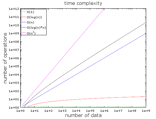
In this figure, you can see the evolution of different types of complexities. I used a logarithmic scale to plot it. In other words, the number of data is quickly increasing from 1 to 1 billion. We can see that:

• The O(1) or constant complexity stays constant (otherwise it wouldn’t be called constant complexity).
• The O(log(n)) stays low even with billions of data.
• The worst complexity is the O(n2) where the number of operations quickly explodes.
• The two other complexities are quickly increasing.

Examples

With a low amount of data, the difference between O(1) and O(n2) is negligible. For example, let’s say you have an algorithm that needs to process 2000 elements.

• An O(1) algorithm will cost you 1 operation
• An O(log(n)) algorithm will cost you 7 operations
• An O(n) algorithm will cost you 2 000 operations
• An O(n*log(n)) algorithm will cost you 14 000 operations
• An O(n2) algorithm will cost you 4 000 000 operations

The difference between O(1) and O(n2) seems a lot (4 million) but you’ll lose at max 2 ms, just the time to blink your eyes. Indeed, current processors can handle hundreds of millions of operations per second . This is why performance and optimization are not an issue in many IT projects.

As I said, it’s still important to know this concept when facing a huge number of data. If this time the algorithm needs to process 1 000 000 elements (which is not that big for a database):

• An O(1) algorithm will cost you 1 operation
• An O(log(n)) algorithm will cost you 14 operations
• An O(n) algorithm will cost you 1 000 000 operations
• An O(n*log(n)) algorithm will cost you 14 000 000 operations
• An O(n2) algorithm will cost you 1 000 000 000 000 operations

I didn’t do the math but I’d say with the O(n2) algorithm you have the time to take a coffee (even a second one!). If you put another 0 on the amount of data, you’ll have the time to take a long nap.

Going deeper

To give you an idea:

• A search in a good hash table gives an element in O(1)
• A search in a well-balanced tree gives a result in O(log(n))
• A search in an array gives a result in O(n)
• The best sorting algorithms have an O(n*log(n)) complexity.
• A bad sorting algorithm has an O(n2) complexity

Note: In the next parts, we’ll see these algorithms and data structures.

There are multiple types of time complexity:

• the average case scenario
• the best case scenario
• and the worst case scenario

The time complexity is often the worst case scenario.

I only talked about time complexity but complexity also works for:

• the memory consumption of an algorithm
• the disk I/O consumption of an algorithm

Of course there are worse complexities than n2, like:

• $n^4$: that sucks! Some of the algorithms I’ll mention have this complexity.
• $3^n$: that sucks even more! One of the algorithms we’re going to see in the middle of this article has this complexity (and it’s really used in many databases).
• factorial n : you’ll never get your results, even with a low amount of data.
• $n^n$: if you end-up with this complexity, you should ask yourself if IT is really your field…

Note: I didn’t give you the real definition of the big O notation but just the idea. You can read this article on Wikipedia for the real (asymptotic) definition.

Merge Sort

What do you do when you need to sort a collection? What? You call the sort() function … ok, good answer… But for a database you have to understand how this sort() function works.

There are several good sorting algorithms so I’ll focus on the most important one: the merge sort. You might not understand right now why sorting data is useful but you should after the part on query optimization. Moreover, understanding the merge sort will help us later to understand a common database join operation called the merge join.

Merge

Like many useful algorithms, the merge sort is based on a trick: merging 2 sorted arrays of size N/2 into a N-element sorted array only costs N operations. This operation is called a merge.

Let’s see what this means with a simple example:

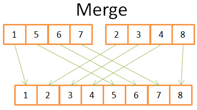
You can see on this figure that to construct the final sorted array of 8 elements, you only need to iterate one time in the 2 4-element arrays. Since both 4-element arrays are already sorted:

• 1. you compare both current elements in the 2 arrays (current=first for the first time)
• 2. then take the lowest one to put it in the 8-element array
• 3. and go to the next element in the array you took the lowest element
• and repeat 1,2,3 until you reach the last element of one of the arrays.
• Then you take the rest of the elements of the other array to put them in the 8-element array.

This works because both 4-element arrays are sorted and therefore you don’t need to “go back” in these arrays.

Now that we’ve understood this trick, here is my pseudocode of the merge sort.

array mergeSort(array a)
   if(length(a)==1)
      return a[0];
   end if
 
   //recursive calls
   [left_array right_array] := split_into_2_equally_sized_arrays(a);
   array new_left_array := mergeSort(left_array);
   array new_right_array := mergeSort(right_array);
 
   //merging the 2 small ordered arrays into a big one
   array result := merge(new_left_array,new_right_array);
   return result;

The merge sort breaks the problem into smaller problems then finds the results of the smaller problems to get the result of the initial problem (note: this kind of algorithms is called divide and conquer). If you don’t understand this algorithm, don’t worry; I didn’t understand it the first time I saw it. If it can help you, I see this algorithm as a two-phase algorithm:

• The division phase where the array is divided into smaller arrays
• The sorting phase where the small arrays are put together (using the merge) to form a bigger array.

Division phase

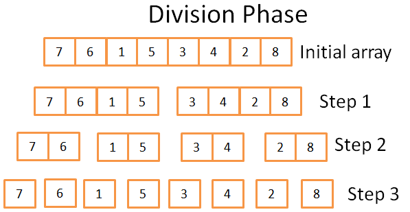
During the division phase, the array is divided into unitary arrays using 3 steps. The formal number of steps is log(N) (since N=8, log(N) = 3).

How do I know that?

I’m a genius! In one word: mathematics. The idea is that each step divides the size of the initial array by 2. The number of steps is the number of times you can divide the initial array by two. This is the exact definition of logarithm (in base 2).

Sorting phase

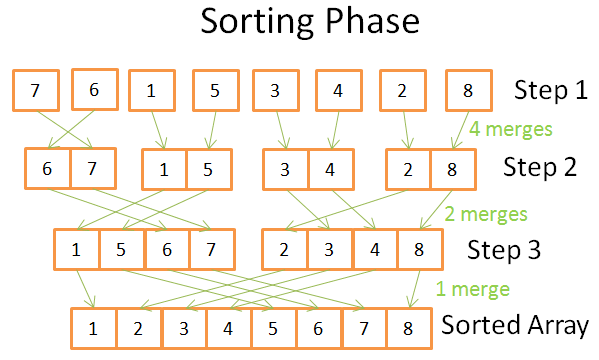
In the sorting phase, you start with the unitary arrays. During each step, you apply multiple merges and the overall cost is N=8 operations:

• In the first step you have 4 merges that cost 2 operations each
• In the second step you have 2 merges that cost 4 operations each
• In the third step you have 1 merge that costs 8 operations

Since there are log(N) steps, the overall costs N * log(N) operations.

The power of the merge sort

Why this algorithm is so powerful?

Because:

• You can modify it in order to reduce the memory footprint, in a way that you don’t create new arrays but you directly modify the input array.

Note: this kind of algorithms is called in-place .

• You can modify it in order to use disk space and a small amount of memory at the same time without a huge disk I/O penalty. The idea is to load in memory only the parts that are currently processed. This is important when you need to sort a multi-gigabyte table with only a memory buffer of 100 megabytes.

Note: this kind of algorithms is called external sorting .

• You can modify it to run on multiple processes/threads/servers.

For example, the distributed merge sort is one of the key components of Hadoop (which is THE framework in Big Data).

T- his algorithm can turn lead into gold (true fact!).

This sorting algorithm is used in most (if not all) databases but it’s not the only one. If you want to know more, you can read this research paper that discusses the pros and cons of the common sorting algorithms in a database.

Array, Tree and Hash table

Now that we understand the idea behind time complexity and sorting, I have to tell you about 3 data structures. It’s important because they’re the backbone of modern databases. I’ll also introduce the notion of database index.

Array

The two-dimensional array is the simplest data structure. A table can be seen as an array. For example:

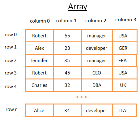
This 2-dimensional array is a table with rows and columns:

• Each row represents a subject
• The columns the features that describe the subjects.
• Each column stores a certain type of data (integer, string, date …).

Though it’s great to store and visualize data, when you need to look for a specific value it sucks.

For example, if you want to find all the guys who work in the UK, you’ll have to look at each row to find if the row belongs to the UK. This will cost you N operations (N being the number of rows) which is not bad but could there be a faster way? This is where trees come into play.

Note: Most modern databases provide advanced arrays to store tables efficiently like heap-organized tables or index-organized tables. But it doesn’t change the problem of fast searching for a specific condition on a group of columns.

Tree and database index

A binary search tree is a binary tree with a special property, the key in each node must be:

• greater than all keys stored in the left sub-tree
• smaller than all keys stored in the right sub-tree

Let’s see what it means visually

The idea

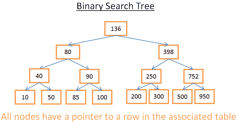
This tree has N=15 elements. Let’s say I’m looking for 208:

• I start with the root whose key is 136. Since 136<208, I look at the right sub-tree of the node 136.
• 398>208 so, I look at the left sub-tree of the node 398
• 250>208 so, I look at the left sub-tree of the node 250
• 200<208 so, I look at the right sub-tree of the node 200. But 200 doesn’t have a right subtree, the value doesn’t exist (because if it did exist it would be in the right subtree of 200)

Now let’s say I’m looking for 40

• I start with the root whose key is 136. Since 136>40, I look at the left sub-tree of the node 136.
• 80>40 so, I look at the left sub-tree of the node 80
• 40= 40, the node exists. I extract the id of the row inside the node (it’s not in the figure) and look at the table for the given row id.
• Knowing the row id let me know where the data is precisely on the table and therefore I can get it instantly.

In the end, both searches cost me the number of levels inside the tree. If you read carefully the part on the merge sort you should see that there are log(N) levels. So the cost of the search is log(N), not bad!

Back to our problem

But this stuff is very abstract so let’s go back to our problem. Instead of a stupid integer, imagine the string that represents the country of someone in the previous table. Suppose you have a tree that contains the column “country” of the table:

• If you want to know who is working in the UK
• you look at the tree to get the node that represents the UK
• inside the “UK node” you’ll find the locations of the rows of the UK workers.

This search only costs you log(N) operations instead of N operations if you directly use the array. What you’ve just imagined was a database index.

You can build a tree index for any group of columns (a string, an integer, 2 strings, an integer and a string, a date …) as long as you have a function to compare the keys (i.e. the group of columns) so that you can establish an order among the keys (which is the case for any basic types in a database).

B+Tree Index

Although this tree works well to get a specific value, there is a BIG problem when you need to get multiple elements between two values. It will cost O(N) because you’ll have to look at each node in the tree and check if it’s between these 2 values (for example, with an in-order traversal of the tree). Moreover this operation is not disk I/O friendly since you’ll have to read the full tree. We need to find a way to efficiently do a range query. To answer this problem, modern databases use a modified version of the previous tree called B+Tree. In a B+Tree:

• only the lowest nodes (the leaves) store information (the location of the rows in the associated table)
• the other nodes are just here to route to the right node during the search.

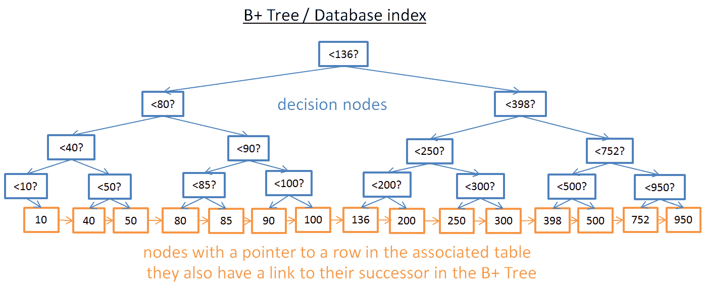
As you can see, there are more nodes (twice more). Indeed, you have additional nodes, the “decision nodes” that will help you to find the right node (that stores the location of the rows in the associated table). But the search complexity is still in O(log(N)) (there is just one more level). The big difference is that the lowest nodes are linked to their successors.

With this B+Tree, if you’re looking for values between 40 and 100:

• You just have to look for 40 (or the closest value after 40 if 40 doesn’t exist) like you did with the previous tree.
• Then gather the successors of 40 using the direct links to the successors until you reach 100.

Let’s say you found M successors and the tree has N nodes. The search for a specific node costs log(N) like the previous tree. But, once you have this node, you get the M successors in M operations with the links to their successors. This search only costs M + log(N) operations vs N operations with the previous tree. Moreover, you don’t need to read the full tree (just M + log(N) nodes), which means less disk usage. If M is low (like 200 rows) and N large (1 000 000 rows) it makes a BIG difference.

But there are new problems (again!). If you add or remove a row in a database (and therefore in the associated B+Tree index):

• you have to keep the order between nodes inside the B+Tree otherwise you won’t be able to find nodes inside the mess.
• you have to keep the lowest possible number of levels in the B+Tree otherwise the time complexity in O(log(N)) will become O(N).

I other words, the B+Tree needs to be self-ordered and self-balanced. Thankfully, this is possible with smart deletion and insertion operations. But this comes with a cost: the insertion and deletion in a B+Tree are in O(log(N)). This is why some of you have heard that using too many indexes is not a good idea. Indeed, you’re slowing down the fast insertion/update/deletion of a row in a table since the database needs to update the indexes of the table with a costly O(log(N)) operation per index. Moreover, adding indexes means more workload for the transaction manager (we will see this manager at the end of the article).

For more details, you can look at the Wikipedia 【article about B+Tree](https://en.wikipedia.org/wiki/B%2B_tree). If you want an example of a B+Tree implementation in a database, look at this article and this article from a core developer of MySQL. They both focus on how innoDB (the engine of MySQL) handles indexes.

Note: I was told by a reader that, because of low-level optimizations, the B+Tree needs to be fully balanced.

Hash table

Our last important data structure is the hash table. It’s very useful when you want to quickly look for values. Moreover, understanding the hash table will help us later to understand a common database join operation called the hash join. This data structure is also used by a database to store some internal stuff (like the lock table or the buffer pool, we’ll see both concepts later)

The hash table is a data structure that quickly finds an element with its key. To build a hash table you need to define:

• a key for your elements
• a hash function for the keys. The computed hashes of the keys give the locations of the elements (called buckets).
• a function to compare the keys. Once you found the right bucket you have to find the element you’re looking for inside the bucket using this comparison.

A simple example

Let’s have a visual example:

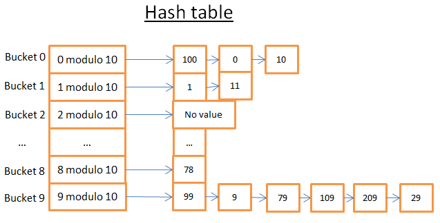
This hash table has 10 buckets. Since I’m lazy I only drew 5 buckets but I know you’re smart so I let you imagine the 5 others. The Hash function I used is the modulo 10 of the key. In other words I only keep the last digit of the key of an element to find its bucket:

• if the last digit is 0 the element ends up in the bucket 0,
• if the last digit is 1 the element ends up in the bucket 1,
• if the last digit is 2 the element ends up in the bucket 2,
• …

The compare function I used is simply the equality between 2 integers.

Let’s say you want to get the element 78:

• The hash table computes the hash code for 78 which is 8.
• It looks in the bucket 8, and the first element it finds is 78.
• It gives you back the element 78
• The search only costs 2 operations (1 for computing the hash value and the other for finding the element inside the bucket).

Now, let’s say you want to get the element 59:

• The hash table computes the hash code for 59 which is 9.
• It looks in the bucket 9, and the first element it finds is 99. Since 99!=59, element 99 is not the right element.
• Using the same logic, it looks at the second element (9), the third (79), … , and the last (29).
• The element doesn’t exist.
• The search costs 7 operations.

A good hash function

As you can see, depending on the value you’re looking for, the cost is not the same!

If I now change the hash function with the modulo 1 000 000 of the key (i.e. taking the last 6 digits), the second search only costs 1 operation because there are no elements in the bucket 000059. The real challenge is to find a good hash function that will create buckets that contain a very small amount of elements.

In my example, finding a good hash function is easy. But this is a simple example, finding a good hash function is more difficult when the key is:

• a string (for example the last name of a person)
• 2 strings (for example the last name and the first name of a person)
• 2 strings and a date (for example the last name, the first name and the birth date of a person)
• …

With a good hash function, the search in a hash table is in O(1).

Array vs hash table

Why not using an array?

Hum, you’re asking a good question.

• A hash table can be half loaded in memory and the other buckets can stay on disk.
• With an array you have to use a contiguous space in memory. If you’re loading a large table it’s very difficult to have enough contiguous space.
• With a hash table you can choose the key you want (for example the country AND the last name of a person).

For more information, you can read my article on the Java HashMap which is an efficient hash table implementation; you don’t need to understand Java to understand the concepts inside this article.

Global overview

We’ve just seen the basic components inside a database. We now need to step back to see the big picture.

A database is a collection of information that can easily be accessed and modified. But a simple bunch of files could do the same. In fact, the simplest databases like SQLite are nothing more than a bunch of files. But SQLite is a well-crafted bunch of files because it allows you to:

• use transactions that ensure data are safe and coherent
• quickly process data even when you’re dealing with millions of data

More generally, a database can be seen as the following figure:

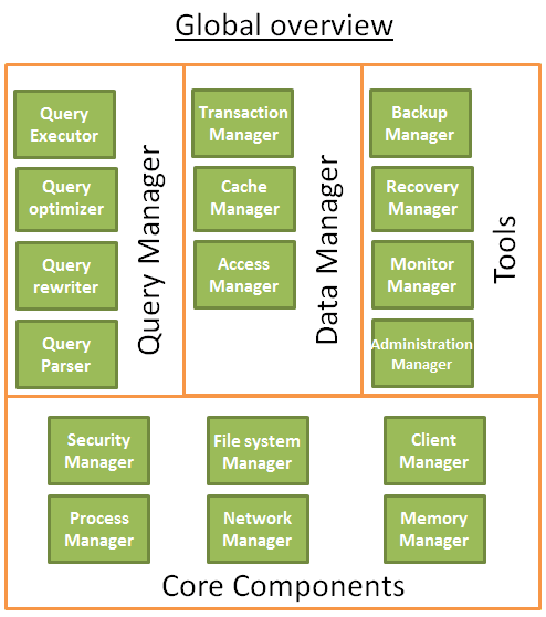
Before writing this part, I’ve read multiple books/papers and every source had its on way to represent a database. So, don’t focus too much on how I organized this database or how I named the processes because I made some choices to fit the plan of this article. What matters are the different components; the overall idea is that a database is divided into multiple components that interact with each other.

The core components:

• The process manager: Many databases have a pool of processes/threads that needs to be managed. Moreover, in order to gain nanoseconds, some modern databases use their own threads instead of the Operating System threads.
• The network manager: Network I/O is a big issue, especially for distributed databases. That’s why some databases have their own manager.
• File system manager: Disk I/O is the first bottleneck of a database. Having a manager that will perfectly handle the Operating System file system or even replace it is important.
• The memory manager: To avoid the disk I/O penalty a large quantity of ram is required. But if you handle a large amount of memory, you need an efficient memory manager. Especially when you have many queries using memory at the same time.
• Security Manager: for managing the authentication and the authorizations of the users
• Client manager: for managing the client connections
• …

The tools:

• Backup manager: for saving and restoring a database.
• Recovery manager: for restarting the database in a coherent state after a crash
• Monitor manager: for logging the activity of the database and providing tools to monitor a database
• Administration manager: for storing metadata (like the names and the structures of the tables) and providing tools to manage databases, schemas, tablespaces, …
• …

The query Manager:

• Query parser: to check if a query is valid
• Query rewriter: to pre-optimize a query
• Query optimizer: to optimize a query
• Query executor: to compile and execute a query

The data manager:

• Transaction manager: to handle transactions
• Cache manager: to put data in memory before using them and put data in memory before writing them on disk
• Data access manager: to access data on disk

For the rest of this article, I’ll focus on how a database manages an SQL query through the following processes:

• the client manager
• the query manager
• the data manager (I’ll also include the recovery manager in this part)

Client manager

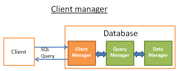
The client manager is the part that handles the communications with the client. The client can be a (web) server or an end-user/end-application. The client manager provides different ways to access the database through a set of well-known APIs: JDBC, ODBC, OLE-DB …

It can also provide proprietary database access APIs.

When you connect to a database:

• The manager first checks your authentication (your login and password) and then checks if you have the authorizations to use the database. These access rights are set by your DBA.
• Then, it checks if there is a process (or a thread) available to manage your query.
• It also checks if the database if not under heavy load.
• It can wait a moment to get the required resources. If this wait reaches a timeout, it closes the connection and gives a readable error message.
• Then it sends your query to the query manager and your query is processed
• Since the query processing is not an “all or nothing” thing, as soon as it gets data from the query manager, it stores the partial results in a buffer and start sending them to you.
• In case of problem, it stops the connection, gives you a readable explanation and releases the resources.

Query manager

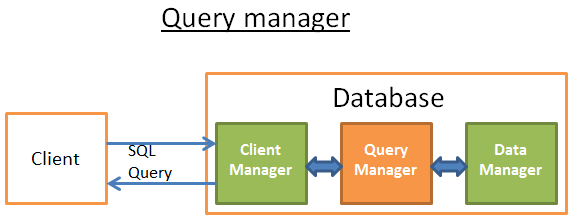
This part is where the power of a database lies. During this part, an ill-written query is transformed into a fast executable code. The code is then executed and the results are returned to the client manager. It’s a multiple-step operation:

• the query is first parsed to see if it’s valid
• it’s then rewritten to remove useless operations and add some pre-optimizations
• it’s then optimized to improve the performances and transformed into an execution and data access plan.
• then the plan is compiled
• at last, it’s executed

In this part, I won’t talk a lot about the last 2 points because they’re less important.

After reading this part, if you want a better understanding I recommend reading:

• The initial research paper (1979) on cost based optimization: Access Path Selection in a Relational Database Management System . - This article is only 12 pages and understandable with an average level in computer science.
• A very good and in-depth presentation on how DB2 9.X optimizes queries here
• A very good presentation on how PostgreSQL optimizes queries here . It’s the most accessible document since it’s more a presentation on “let’s see what query plans PostgreSQL gives in these situations“ than a “let’s see the algorithms used by PostgreSQL”.
• The official SQLite documentation about optimization. It’s “easy” to read because SQLite uses simple rules. Moreover, it’s the only official documentation that really explains how it works.
• A good presentation on how SQL Server 2005 optimizes queries here
• A white paper about optimization in Oracle 12c here
• 2 theoretical courses on query optimization from the authors of the book “DATABASE SYSTEM CONCEPTS” here and here . A good read that focuses on disk I/O cost but a good level in CS is required.
• Another theoretical course that I find more accessible but that only focuses on join operators and disk I/O.

Query parser

Each SQL statement is sent to the parser where it is checked for correct syntax. If you made a mistake in your query the parser will reject the query. For example, if you wrote “SLECT …” instead of “SELECT …”, the story ends here.

But this goes deeper. It also checks that the keywords are used in the right order. For example a WHERE before a SELECT will be rejected.

Then, the tables and the fields inside the query are analyzed. The parser uses the metadata of the database to check:

• If the tables exist
• If the fields of the tables exist
• If the operations for the types of the fields are possible (for example you can’t compare an integer with a string, you can’t use a substring() function on an integer)

Then it checks if you have the authorizations to read (or write) the tables in the query. Again, these access rights on tables are set by your DBA.

During this parsing, the SQL query is transformed into an internal representation (often a tree)

If everything is ok then the internal representation is sent to the query rewriter.

Query rewriter

At this step, we have an internal representation of a query. The aim of the rewriter is:

• to pre-optimize the query
• to avoid unnecessary operations
• to help the optimizer to find the best possible solution

The rewriter executes a list of known rules on the query. If the query fits a pattern of a rule, the rule is applied and the query is rewritten. Here is a non-exhaustive list of (optional) rules:

• View merging: If you’re using a view in your query, the view is transformed with the SQL code of the view.
• Subquery flattening: Having subqueries is very difficult to optimize so the rewriter will try to modify a query with a subquery to remove the subquery.

For example

SELECT PERSON.*
FROM PERSON
WHERE PERSON.person_key IN
(SELECT MAILS.person_key
FROM MAILS
WHERE MAILS.mail LIKE 'christophe%');

Will be replaced by

SELECT PERSON.*
FROM PERSON, MAILS
WHERE PERSON.person_key = MAILS.person_key
and MAILS.mail LIKE 'christophe%';

• Removal of unnecessary operators: For example if you use a DISTINCT whereas you have a UNIQUE constraint that prevents the data from being non-unique, the DISTINCT keyword is removed.
• Redundant join elimination: If you have twice the same join condition because one join condition is hidden in a view or if by transitivity there is a useless join, it’s removed.
• Constant arithmetic evaluation: If you write something that requires a calculus, then it’s computed once during the rewriting. For example WHERE AGE > 10+2 is transformed into WHERE AGE > 12 and TODATE(“some date”) is transformed into the date in the datetime format
• (Advanced) Partition Pruning: If you’re using a partitioned table, the rewriter is able to find what partitions to use.
• (Advanced) Materialized view rewrite: If you have a materialized view that matches a subset of the predicates in your query, the rewriter checks if the view is up to date and modifies the query to use the materialized view instead of the raw tables.
• (Advanced) Custom rules: If you have custom rules to modify a query (like Oracle policies), then the rewriter executes these rules
• (Advanced) Olap transformations: analytical/windowing functions, star joins, rollup … are also transformed (but I’m not sure if it’s done by the rewriter or the optimizer, since both processes are very close it must depends on the database).

This rewritten query is then sent to the query optimizer where the fun begins!

Statistics

Before we see how a database optimizes a query we need to speak about statistics because without them a database is stupid. If you don’t tell the database to analyze its own data, it will not do it and it will make (very) bad assumptions.

But what kind of information does a database need?

I have to (briefly) talk about how databases and Operating systems store data. They’re using a minimum unit called a page or a block (4 or 8 kilobytes by default). This means that if you only need 1 Kbytes it will cost you one page anyway. If the page takes 8 Kbytes then you’ll waste 7 Kbytes.

Back to the statistics! When you ask a database to gather statistics, it computes values like:

• The number of rows/pages in a table
• For each column in a table:
  • distinct data values
  • the length of data values (min, max, average)
  • data range information (min, max, average)
• Information on the indexes of the table.

These statistics will help the optimizer to estimate the disk I/O, CPU and memory usages of the query.

The statistics for each column are very important. For example if a table PERSON needs to be joined on 2 columns: LAST_NAME, FIRST_NAME. With the statistics, the database knows that there are only 1 000 different values on FIRST_NAME and 1 000 000 different values on LAST_NAME. Therefore, the database will join the data on LAST_NAME, FIRST_NAME instead of FIRST_NAME,LAST_NAME because it produces way less comparisons since the LAST_NAME are unlikely to be the same so most of the time a comparison on the 2 (or 3) first characters of the LAST_NAME is enough.

But these are basic statistics. You can ask a database to compute advanced statistics called histograms. Histograms are statistics that inform about the distribution of the values inside the columns. For example

• the most frequent values
• the quantiles
• …

These extra statistics will help the database to find an even better query plan. Especially for equality predicate (ex: WHERE AGE = 18 ) or range predicates (ex: WHERE AGE > 10 and AGE <40 ) because the database will have a better idea of the number rows concerned by these predicates (note: the technical word for this concept is selectivity).

The statistics are stored in the metadata of the database. For example you can see the statistics for the (non-partitioned) tables:

• in USER/ALL/DBA_TABLES and USER/ALL/DBA_TAB_COLUMNS for Oracle
• in SYSCAT.TABLES and SYSCAT.COLUMNS for DB2.

The statistics have to be up to date. There is nothing worse than a database thinking a table has only 500 rows whereas it has 1 000 000 rows. The only drawback of the statistics is that it takes time to compute them. This is why they’re not automatically computed by default in most databases. It becomes difficult with millions of data to compute them. In this case, you can choose to compute only the basics statistics or to compute the stats on a sample of the database.

For example, when I was working on a project dealing with hundreds of millions rows in each tables, I chose to compute the statistics on only 10%, which led to a huge gain in time. For the story it turned out to be a bad decision because occasionally the 10% chosen by Oracle 10G for a specific column of a specific table were very different from the overall 100% (which is very unlikely to happen for a table with 100M rows). This wrong statistic led to a query taking occasionally 8 hours instead of 30 seconds; a nightmare to find the root cause. This example shows how important the statistics are.

Note: Of course, there are more advanced statistics specific for each database. If you want to know more, read the documentations of the databases. That being said, I’ve tried to understand how the statistics are used and the best official documentation I found was the one from PostgreSQL .

Query optimizer

All modern databases are using a Cost Based Optimization (or CBO) to optimize queries. The idea is to put a cost an every operation and find the best way to reduce the cost of the query by using the cheapest chain of operations to get the result.

To understand how a cost optimizer works I think it’s good to have an example to “feel” the complexity behind this task. In this part I’ll present you the 3 common ways to join 2 tables and we will quickly see that even a simple join query is a nightmare to optimize. After that, we’ll see how real optimizers do this job.

For these joins, I’ll focus on their time complexity but a database optimizer computes their CPU cost, disk I/O cost and memory requirement. The difference between time complexity and CPU cost is that time cost is very approximate (it’s for lazy guys like me). For the CPU cost, I should count every operation like an addition, an “if statement”, a multiplication, an iteration … Moreover:

• Each high level code operation has a specific number of low level CPU operations.
• The cost of a CPU operation is not the same (in terms of CPU cycles) whether you’re using an Intel Core i7, an Intel Pentium 4, an AMD Opteron…. In other words it depends on the CPU architecture.

Using the time complexity is easier (at least for me) and with it we can still get the concept of CBO. I’ll sometimes speak about disk I/O since it’s an important concept. Keep in mind that the bottleneck is most of the time the disk I/O and not the CPU usage.

Indexes

We talked about indexes when we saw the B+Trees. Just remember that these indexes are already sorted.

FYI, there are other types of indexes like bitmap indexes. They don’t offer the same cost in terms of CPU, disk I/O and memory than B+Tree indexes.

Moreover, many modern databases can dynamically create temporary indexes just for the current query if it can improve the cost of the execution plan.

Access Path

Before applying your join operators, you first need to get your data. Here is how you can get your data.

Note: Since the real problem with all the access paths is the disk I/O, I won’t talk a lot about time complexity.

Full scan

If you’ve ever read an execution plan you must have seen the word full scan (or just scan). A full scan is simply the database reading a table or an index entirely. In terms of disk I/O, a table full scan is obviously more expensive than an index full scan.

Range Scan

There are other types of scan like index range scan. It is used for example when you use a predicate like “WHERE AGE > 20 AND AGE <40”.

Of course you need have an index on the field AGE to use this index range scan.

We already saw in the first part that the time cost of a range query is something like log(N) +M, where N is the number of data in this index and M an estimation of the number of rows inside this range. Both N and M values are known thanks to the statistics (Note: M is the selectivity for the predicate AGE >20 AND AGE<40). Moreover, for a range scan you don’t need to read the full index so it’s less expensive in terms of disk I/O than a full scan.

Unique scan

If you only need one value from an index you can use the unique scan.

Access by row id

Most of the time, if the database uses an index, it will have to look for the rows associated to the index. To do so it will use an access by row id.

For example, if you do something like

SELECT LASTNAME, FIRSTNAME from PERSON WHERE AGE = 28

If you have an index for person on column age, the optimizer will use the index to find all the persons who are 28 then it will ask for the associate rows in the table because the index only has information about the age and you want to know the lastname and the firstname.

But, if now you do something like

SELECT TYPE_PERSON.CATEGORY from PERSON ,TYPE_PERSON
WHERE PERSON.AGE = TYPE_PERSON.AGE

The index on PERSON will be used to join with TYPE_PERSON but the table PERSON will not be accessed by row id since you’re not asking information on this table.

Though it works great for a few accesses, the real issue with this operation is the disk I/O. If you need too many accesses by row id the database might choose a full scan.

Others paths

I didn’t present all the access paths. If you want to know more, you can read the Oracle documentation . The names might not be the same for the other databases but the concepts behind are the same.

Join operators

So, we know how to get our data, let’s join them!

I’ll present the 3 common join operators: Merge Join, Hash Join and Nested Loop Join. But before that, I need to introduce new vocabulary: inner relation and outer relation. A relation can be:

• a table
• an index
• an intermediate result from a previous operation (for example the result of a previous join)

When you’re joining two relations, the join algorithms manage the two relations differently. In the rest of the article, I’ll assume that:

• the outer relation is the left data set
• the inner relation is the right data set

For example, A JOIN B is the join between A and B where A is the outer relation and B the inner relation.

Most of the time, the cost of A JOIN B is not the same as the cost of B JOIN A.

In this part, I’ll also assume that the outer relation has N elements and the inner relation M elements. Keep in mind that a real optimizer knows the values of N and M with the statistics.

Note: N and M are the cardinalities of the relations.

Nested loop join

The nested loop join is the easiest one.

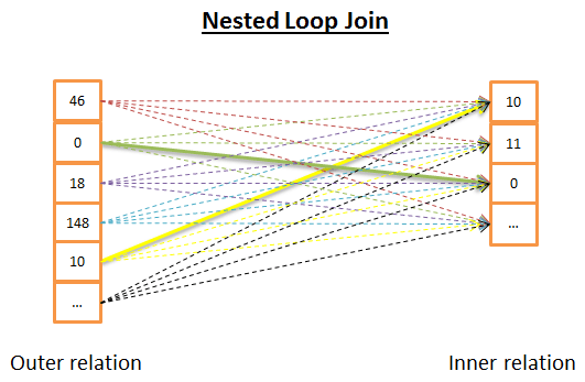
Here is the idea:

• for each row in the outer relation
• you look at all the rows in the inner relation to see if there are rows that match

Here is a pseudo code:

nested_loop_join(array outer, array inner)
  for each row a in outer
    for each row b in inner
      if (match_join_condition(a,b))
        write_result_in_output(a,b)
      end if
    end for
   end for

Since it’s a double iteration, the time complexity is O(N*M)

In term of disk I/O, for each of the N rows in the outer relation, the inner loop needs to read M rows from the inner relation. This algorithm needs to read N + N*M rows from disk. But, if the inner relation is small enough, you can put the relation in memory and just have M +N reads. With this modification, the inner relation must be the smallest one since it has more chance to fit in memory.

In terms of time complexity it makes no difference but in terms of disk I/O it’s way better to read only once both relations.

Of course, the inner relation can be replaced by an index, it will be better for the disk I/O.

Since this algorithm is very simple, here is another version that is more disk I/O friendly if the inner relation is too big to fit in memory. Here is the idea:

• instead of reading both relation row by row,
• you read them bunch by bunch and keep 2 bunches of rows (from each relation) in memory,
• you compare the rows inside the two bunches and keep the rows that match,
• then you load new bunches from disk and compare them
• and so on until there are no bunches to load.

Here is a possible algorithm:

// improved version to reduce the disk I/O.
nested_loop_join_v2(file outer, file inner)
  for each bunch ba in outer
  // ba is now in memory
    for each bunch bb in inner
        // bb is now in memory
        for each row a in ba
          for each row b in bb
            if (match_join_condition(a,b))
              write_result_in_output(a,b)
            end if
          end for
       end for
    end for
   end for

With this version, the time complexity remains the same, but the number of disk access decreases:

• With the previous version, the algorithm needs N + N*M accesses (each access gets one row).
• With this new version, the number of disk accesses becomes number_of_bunches_for(outer)+ number_of_ bunches_for(outer)* number_of_ bunches_for(inner).
• If you increase the size of the bunch you reduce the number of disk accesses.

Note: Each disk access gathers more data than the previous algorithm but it doesn’t matter since they’re sequential accesses (the real issue with mechanical disks is the time to get the first data).

Hash join

The hash join is more complicated but gives a better cost than a nested loop join in many situations.

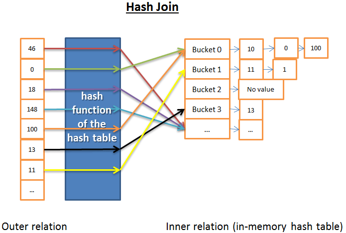
The idea of the hash join is to:

• 1. Get all elements from the inner relation
• 2. Build an in-memory hash table
• 3. Get all elements of the outer relation one by one
• 4. Compute the hash of each element (with the hash function of the hash table) to find the associated bucket of the inner relation
• 5. find if there is a match between the elements in the bucket and the element of the outer table

In terms of time complexity I need to make some assumptions to simplify the problem:

• The inner relation is divided into X buckets
• The hash function distributes hash values almost uniformly for both relations. In other words the buckets are equally sized.
• The matching between an element of the outer relation and all elements inside a bucket costs the number of elements inside the buckets.

The time complexity is (M/X) * N + cost_to_create_hash_table(M) + cost_of_hash_function*N

If the Hash function creates enough small-sized buckets then the time complexity is O(M+N)

Here is another version of the hash join which is more memory friendly but less disk I/O friendly. This time:

• 1. you compute the hash tables for both the inner and outer relations
• 2. then you put them on disk
• 3. then you compare the 2 relations bucket by bucket (with one loaded in-memory and the other read row by row)

Merge join

The merge join is the only join that produces a sorted result.

Note: In this simplified merge join, there are no inner or outer tables; they both play the same role. But real implementations make a difference, for example, when dealing with duplicates.

The merge join can be divided into of two steps:

1. (Optional) Sort join operations: Both the inputs are sorted on the join key(s).
2. Merge join operation: The sorted inputs are merged together.

Sort

We already spoke about the merge sort, in this case a merge sort in a good algorithm (but not the best if memory is not an issue).

But sometimes the data sets are already sorted, for example:

• If the table is natively ordered, for example an index-organized table on the join condition
• If the relation is an index on the join condition
• If this join is applied on an intermediate result already sorted during the process of the query

Merge join

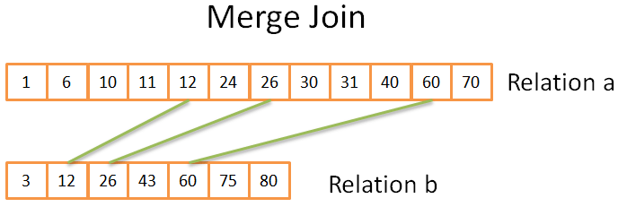
This part is very similar to the merge operation of the merge sort we saw. But this time, instead of picking every element from both relations, we only pick the elements from both relations that are equals. Here is the idea:

• 1. you compare both current elements in the 2 relations (current=first for the first time)
• 2. if they’re equal, then you put both elements in the result and you go to the next element for both relations
• 3. if not, you go to the next element for the relation with the lowest element (because the next element might match)
• 4. and repeat 1,2,3 until you reach the last element of one of the relation.

This works because both relations are sorted and therefore you don’t need to “go back” in these relations.

This algorithm is a simplified version because it doesn’t handle the case where the same data appears multiple times in both arrays (in other words a multiple matches). The real version is more complicated “just” for this case; this is why I chose a simplified version.

If both relations are already sorted then the time complexity is O(N+M)

If both relations need to be sorted then the time complexity is the cost to sort both relations: O(N*Log(N) + M*Log(M))

For the CS geeks, here is a possible algorithm that handles the multiple matches (note: I’m not 100% sure about my algorithm):

mergeJoin(relation a, relation b)
  relation output
  integer a_key:=0;
  integer b_key:=0;
  
  while (a[a_key]!=null or b[b_key]!=null)
    if (a[a_key] < b[b_key])
      a_key++;
    else if (a[a_key] > b[b_key])
      b_key++;
    else //Join predicate satisfied
    //i.e. a[a_key] == b[b_key]
 
      //count the number of duplicates in relation a
      integer nb_dup_in_a = 1:
      while (a[a_key]==a[a_key+nb_dup_in_a])
        nb_dup_in_a++;
         
      //count the number of duplicates in relation b
      integer dup_in_b = 1:
      while (b[b_key]==b[b_key+nb_dup_in_b])
        nb_dup_in_b++;
         
      //write the duplicates in output
       for (int i = 0 ; i< nb_dup_in_a ; i++)
         for (int j = 0 ; i< nb_dup_in_b ; i++)     
           write_result_in_output(a[a_key+i],b[b_key+j])
            
      a_key=a_key + nb_dup_in_a-1;
      b_key=b_key + nb_dup_in_b-1;
 
    end if
  end while

Which one is the best?

If there was a best type of joins, there wouldn’t be multiple types. This question is very difficult because many factors come into play like:

• The amount of free memory: without enough memory you can say goodbye to the powerful hash join (at least the full in-memory hash join)
• The size of the 2 data sets. For example if you have a big table with a very small one, a nested loop join will be faster than a hash join because the hash join has an expensive creation of hashes. If you have 2 very large tables the nested loop join will be very CPU expensive.
• The presence of indexes. With 2 B+Tree indexes the smart choice seems to be the merge join
• If the result need to be sorted: Even if you’re working with unsorted data sets, you might want to use a costly merge join (with the sorts) because at the end the result will be sorted and you’ll be able to chain the result with another merge join (or maybe because the query asks implicitly/explicitly for a sorted result with an ORDER BY/GROUP BY/DISTINCT operation)
• If the relations are already sorted: In this case the merge join is the best candidate
• The type of joins you’re doing: is it an equijoin (i.e.: tableA.col1 = tableB.col2)? Is it an inner join, an outer join, a cartesian product or a self-join? Some joins can’t work in certain situations.
• The distribution of data. If the data on the join condition are skewed (For example you’re joining people on their last name but many people have the same), using a hash join will be a disaster because the hash function will create ill-distributed buckets. If you want the join to be executed by multiple threads/process

For more information, you can read the DB2 , ORACLE or SQL Server documentations.

Simplified example

We’ve just seen 3 types of join operations.

Now let’s say we need to join 5 tables to have a full view of a person. A PERSON can have:

• multiple MOBILES
• multiple MAILS
• multiple ADRESSES
• multiple BANK_ACCOUNTS

In other words we need a quick answer for the following query:

SELECT * from PERSON, MOBILES, MAILS,ADRESSES, BANK_ACCOUNTS
WHERE
PERSON.PERSON_ID = MOBILES.PERSON_ID
AND PERSON.PERSON_ID = MAILS.PERSON_ID
AND PERSON.PERSON_ID = ADRESSES.PERSON_ID
AND PERSON.PERSON_ID = BANK_ACCOUNTS.PERSON_ID

As a query optimizer, I have to find the best way to process the data. But there are 2 problems:

• What kind of join should I use for each join?

I have 3 possible joins (Hash Join, Merge Join, Nested Join) with the possibility to use 0,1 or 2 indexes (not to mention that there are different types of indexes).

• What order should I choose to compute the join?

For example, the following figure shows different possible plans for only 3 joins on 4 tables

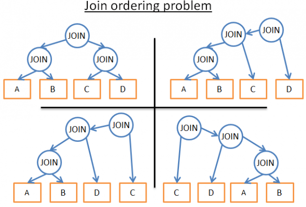
So here are my possibilities:

• 1. I use a brute force approach Using the database statistics, I compute the cost for every possible plan and I keep the best one. But there are many possibilities. For a given order of joins, each join has 3 possibilities: HashJoin, MergeJoin, NestedJoin. So, for a given order of joins there are $3^4$ possibilities. The join ordering is a permutation problem on a binary tree and there are (2*4)!/(4+1)! possible orders. For this very simplified problem, I end up with $3^4$*(2*4)!/(4+1)! possibilities.

In non-geek terms, it means 27 216 possible plans. If I now add the possibility for the merge join to take 0,1 or 2 B+Tree indexes, the number of possible plans becomes 210 000. Did I forget to mention that this query is VERY SIMPLE?

• 2. I cry and quit this job

It’s very tempting but you wouldn’t get your result and I need money to pay the bills.

• 3. I only try a few plans and take the one with the lowest cost.

Since I’m not superman, I can’t compute the cost of every plan. Instead, I can arbitrary choose a subset of all the possible plans, compute their costs and give you the best plan of this subset.

• 4. I apply smart rules to reduce the number of possible plans.

There are 2 types of rules:

I can use “logical” rules that will remove useless possibilities but they won’t filter a lot of possible plans. For example: “the inner relation of the nested loop join must be the smallest data set”

I accept not finding the best solution and apply more aggressive rules to reduce a lot the number of possibilities. For example “If a relation is small, use a nested loop join and never use a merge join or a hash join”

In this simple example, I end up with many possibilities. But a real query can have other relational operators like OUTER JOIN, CROSS JOIN, GROUP BY, ORDER BY, PROJECTION, UNION, INTERSECT, DISTINCT … which means even more possibilities.

So, how a database does it?

Dynamic programming, greedy algorithm and heuristic

A relational database tries the multiple approaches I’ve just said. The real job of an optimizer is to find a good solution on a limited amount of time.

Most of the time an optimizer doesn’t find the best solution but a “good” one.

For small queries, doing a brute force approach is possible. But there is a way to avoid unnecessary computations so that even medium queries can use the brute force approach. This is called dynamic programming.

Dynamic Programming

The idea behind these 2 words is that many executions plan are very similar. If you look at the following plans:

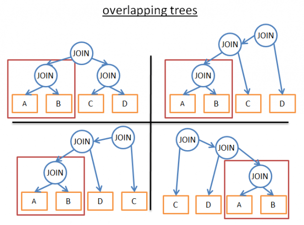
They share the same (A JOIN B) subtree. So, instead of computing the cost of this subtree in every plan, we can compute it once, save the computed cost and reuse it when we see this subtree again. More formally, we’re facing an overlapping problem. To avoid the extra-computation of the partial results we’re using memoization.

Using this technique, instead of having a (2*N)!/(N+1)! time complexity, we “just” have $3^N$. In our previous example with 4 joins, it means passing from 336 ordering to 81. If you take a bigger query with 8 joins (which is not big), it means passing from 57 657 600 to 6561.

For the CS geeks, here is an algorithm I found on the formal course I already gave you . I won’t explain this algorithm so read it only if you already know dynamic programming or if you’re good with algorithms (you’ve been warned!):

procedure findbestplan(S)
if (bestplan[S].cost infinite)
   return bestplan[S]
// else bestplan[S] has not been computed earlier, compute it now
if (S contains only 1 relation)
         set bestplan[S].plan and bestplan[S].cost based on the best way
         of accessing S  /* Using selections on S and indices on S */
     else for each non-empty subset S1 of S such that S1 != S
   P1= findbestplan(S1)
   P2= findbestplan(S - S1)
   A = best algorithm for joining results of P1 and P2
   cost = P1.cost + P2.cost + cost of A
   if cost < bestplan[S].cost
       bestplan[S].cost = cost
      bestplan[S].plan = “execute P1.plan; execute P2.plan;
                 join results of P1 and P2 using A”
return bestplan[S]

For bigger queries you can still do a dynamic programming approach but with extra rules (or heuristics) to remove possibilities:

• If we analyze only a certain type of plan (for example: the left-deep trees) we end up with $n*2^n$ instead of $3^n$

• If we add logical rules to avoid plans for some patterns (like “if a table as an index for the given predicate, don’t try a merge join on the table but only on the index”) it will reduce the number of possibilities without hurting to much the best possible solution.
• If we add rules on the flow (like “perform the join operations BEFORE all the other relational operations”) it also reduces a lot of possibilities.
• …

Greedy algorithms

But for a very big query or to have a very fast answer (but not a very fast query), another type of algorithms is used, the greedy algorithms.

The idea is to follow a rule (or heuristic) to build a query plan in an incremental way. With this rule, a greedy algorithm finds the best solution to a problem one step at a time. The algorithm starts the query plan with one JOIN. Then, at each step, the algorithm adds a new JOIN to the query plan using the same rule.

Let’s take a simple example. Let’s say we have a query with 4 joins on 5 tables (A, B, C, D and E). To simplify the problem we just take the nested join as a possible join. Let’s use the rule “use the join with the lowest cost”

• we arbitrary start on one of the 5 tables (let’s choose A)
• we compute the cost of every join with A (A being the inner or outer relation).
• we find that A JOIN B gives the lowest cost.
• we then compute the cost of every join with the result of A JOIN B (A JOIN B being the inner or outer relation).
• we find that (A JOIN B) JOIN C gives the best cost.
• we then compute the cost of every join with the result of the (A JOIN B) JOIN C …
• ….
• At the end we find the plan (((A JOIN B) JOIN C) JOIN D) JOIN E)

Since we arbitrary started with A, we can apply the same algorithm for B, then C then D then E. We then keep the plan with the lowest cost.

By the way, this algorithm has a name: it’s called the Nearest neighbor algorithm .

I won’t go into details, but with a good modeling and a sort in N*log(N) this problem can easily be solved . The cost of this algorithm is in O(N*log(N)) vs O($3^N$) for the full dynamic programming version. If you have a big query with 20 joins, it means 26 vs 3 486 784 401, a BIG difference!

The problem with this algorithm is that we assume that finding the best join between 2 tables will give us the best cost if we keep this join and add a new join. But:

• even if A JOIN B gives the best cost between A, B and C
• (A JOIN C) JOIN B might give a better result than (A JOIN B) JOIN C.

To improve the result, you can run multiple greedy algorithms using different rules and keep the best plan.

Other algorithms

[If you’re already fed up with algorithms, skip to the next part, what I’m going to say is not important for the rest of the article]

The problem of finding the best possible plan is an active research topic for many CS researchers. They often try to find better solutions for more precise problems/patterns. For example,

• if the query is a star join (it’s a certain type of multiple-join query), some databases will use a specific algorithm.
• if the query is a parallel query, some databases will use a specific algorithm
• …

Other algorithms are also studied to replace dynamic programming for large queries. Greedy algorithms belong to larger family called heuristic algorithms. A greedy algorithm follows a rule (or heuristic), keeps the solution it found at the previous step and “appends” it to find the solution for the current step. Some algorithms follow a rule and apply it in a step-by-step way but don’t always keep the best solution found in the previous step. They are called heuristic algorithms.

For example, genetic algorithms follow a rule but the best solution of the last step is not often kept:

• A solution represents a possible full query plan
• Instead of one solution (i.e. plan) there are P solutions (i.e. plans) kept at each step.
• 0. P query plans are randomly created
• 1. Only the plans with the best costs are kept
• 2. These best plans are mixed up to produce P news plans
• 3. Some of the P new plans are randomly modified
• 4. The step 1,2,3 are repeated T times
• 5. Then you keep the best plan from the P plans of the last loop.

The more loops you do the better the plan will be.

Is it magic? No, it’s the laws of nature: only the fittest survives!

FYI, genetic algorithms are implemented in PostgreSQL but I wasn’t able to find if they’re used by default.

There are other heuristic algorithms used in databases like Simulated Annealing, Iterative Improvement, Two-Phase Optimization… But I don’t know if they’re currently used in enterprise databases or if they’re only used in research databases.

For more information, you can read the following research article that presents more possible algorithms: Review of Algorithms for the Join Ordering Problem in Database Query Optimization

Real optimizers

[You can skip to the next part, what I’m going to say is not important]

But, all this blabla is very theoretical. Since I’m a developer and not a researcher, I like concrete examples.

Let’s see how the SQLite optimizer works. It’s a light database so it uses a simple optimization based on a greedy algorithm with extra-rules to limit the number of possibilities:

• SQLite chooses to never reorder tables in a CROSS JOIN operator -** joins are implemented as nested joins**
• outer joins are always evaluated in the order in which they occur
• …
• Prior to version 3.8.0, SQLite uses the “Nearest Neighbor” greedy algorithm when searching for the best query plan

Wait a minute … we’ve already seen this algorithm! What a coincidence!

• Since version 3.8.0 (released in 2015), SQLite uses the “N Nearest Neighbors ” greedy algorithm when searching for the best query plan

Let’s see how another optimizer does his job. IBM DB2 is like all the enterprise databases but I’ll focus on this one since it’s the last one I’ve really used before switching to Big Data.

If we look at the official documentation , we learn that the DB2 optimizer let you use 7 different levels of optimization:

• Use greedy algorithms for the joins
  • 0 – minimal optimization, use index scan and nested-loop join and avoid some Query Rewrite
  • 1 – low optimization
  • 2 – full optimization
• Use dynamic programming for the joins
  • 3 – moderate optimization and rough approximation
  • 5 – full optimization, uses all techniques with heuristics
  • 7 – full optimization similar to 5, without heuristics
  • 9 – maximal optimization spare no effort/expense considers all possible join orders, including Cartesian products

We can see that DB2 uses greedy algorithms and dynamic programming. Of course, they don’t share the heuristics they use since the query optimizer is the main power of a database.

FYI, the default level is 5. By default the optimizer uses the following characteristics:

• All available statistics, including frequent-value and quantile statistics, are used.
• All query rewrite rules (including materialized query table routing) are applied, except computationally intensive rules that are applicable only in very rare cases.
• Dynamic programming join enumeration is used, with:
  • Limited use of composite inner relation
  • Limited use of Cartesian products for star schemas involving lookup tables
• A wide range of access methods is considered, including list prefetch (note: will see what is means), index ANDing (note: a special operation with indexes), and materialized query table routing.

By default, DB2 uses dynamic programming limited by heuristics for the join ordering.

The others conditions (GROUP BY, DISTINCT…) are handled by simple rules.

Query Plan Cache

Since the creation of a plan takes time, most databases store the plan into a query plan cache to avoid useless re-computations of the same query plan. It’s kind of a big topic since the database needs to know when to update the outdated plans. The idea is to put a threshold and if the statistics of a table have changed above this threshold then the query plan involving this table is purged from the cache.

Query executor

At this stage we have an optimized execution plan. This plan is compiled to become an executable code. Then, if there are enough resources (memory, CPU) it is executed by the query executor. The operators in the plan (JOIN, SORT BY …) can be executed in a sequential or parallel way; it’s up to the executor. To get and write its data, the query executor interacts with the data manager, which is the next part of the article.

Data manager

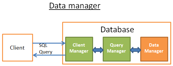
At this step, the query manager is executing the query and needs the data from the tables and indexes. It asks the data manager to get the data, but there are 2 problems:

• Relational databases use a transactional model. So, you can’t get any data at any time because someone else might be using/modifying the data at the same time.
• Data retrieval is the slowest operation in a database, therefore the data manager needs to be smart enough to get and keep data in memory buffers.

In this part, we’ll see how relational databases handle these 2 problems. I won’t talk about the way the data manager gets its data because it’s not the most important (and this article is long enough!).

Cache manager

As I already said, the main bottleneck of databases is disk I/O. To improve performance, modern databases use a cache manager.

Instead of directly getting the data from the file system, the query executor asks for the data to the cache manager. The cache manager has an in-memory cache called buffer pool. Getting data from memory dramatically speeds up a database. It’s difficult to give an order of magnitude because it depends on the operation you need to do:

• sequential access (ex: full scan) vs random access (ex: access by row id),
• read vs write

and the type of disks used by the database:

• 7.2k/10k/15k rpm HDD
• SSD
• RAID 1/5/…

but I’d say memory is 100 to 100k times faster than disk.

But, this leads to another problem (as always with databases…). The cache manager needs to get the data in memory BEFORE the query executor uses them; otherwise the query manager has to wait for the data from the slow disks.

Prefetching

This problem is called prefetching. A query executor knows the data it’ll need because it knows the full flow of the query and has knowledge of the data on disk with the statistics. Here is the idea:

• When the query executor is processing its first bunch of data
• It asks the cache manager to pre-load the second bunch of data
• When it starts processing the second bunch of data
• It asks the CM to pre-load the third bunch and informs the CM that the first bunch can be purged from cache.
• …

The CM stores all these data in its buffer pool. In order to know if a data is still needed, the cache manager adds an extra-information about the cached data (called a latch).

Sometimes the query executor doesn’t know what data it’ll need and some databases don’t provide this functionality. Instead, they use a speculative prefetching (for example: if the query executor asked for data 1,3,5 it’ll likely ask for 7,9,11 in a near future) or a sequential prefetching (in this case the CM simply loads from disks the next contiguous data after the ones asked).

To monitor how well the prefetching is working, modern databases provide a metric called buffer/cache hit ratio. The hit ratio shows how often a requested data has been found in the buffer cache without requiring disk access.

Note: a poor cache hit ratio doesn’t always mean that the cache is ill-working. For more information, you can read the Oracle documentation .

But, a buffer is a limited amount of memory. Therefore, it needs to remove some data to be able to load new ones. Loading and purging the cache has a cost in terms of disk and network I/O. If you have a query that is often executed, it wouldn’t be efficient to always load then purge the data used by this query. To handle this problem, modern databases use a buffer replacement strategy.

Buffer-Replacement strategies

Most modern databases (at least SQL Server, MySQL, Oracle and DB2) use an LRU algorithm.

LRU

LRU stands for Least Recently Used. The idea behind this algorithm is to keep in the cache the data that have been recently used and, therefore, are more likely to be used again.

Here is a visual example:

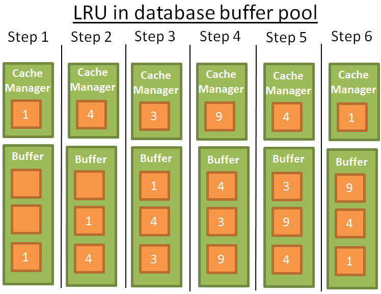
For the sake of comprehension, I’ll assume that the data in the buffer are not locked by latches (and therefore can be removed). In this simple example the buffer can store 3 elements:

• 1: the cache manager uses the data 1 and puts the data into the empty buffer
• 2: the CM uses the data 4 and puts the data into the half-loaded buffer
• 3: the CM uses the data 3 and puts the data into the half-loaded buffer
• 4: the CM uses the data 9. The buffer is full so data 1 is removed since it’s the last recently used data. Data 9 is added into the buffer
• 5: the CM uses the data 4. Data 4 is already in the buffer therefore it becomes the first recently used data again.
• 6: the CM uses the data 1. The buffer is full so data 9 is removed since it’s the last recently used data. Data 1 is added into the buffer
• … This algorithm works well but there are some limitations. What if there is a full scan on a large table? In other words, what happens when the size of the table/index is above the size of the buffer? Using this algorithm will remove all the previous values in the cache whereas the data from the full scan are likely to be used only once.

Improvements

To prevent this to happen, some databases add specific rules. For example according to Oracle documentation :

“For very large tables, the database typically uses a direct path read, which loads blocks directly […], to avoid populating the buffer cache. For medium size tables, the database may use a direct read or a cache read. If it decides to use a cache read, then the database places the blocks at the end of the LRU list to prevent the scan from effectively cleaning out the buffer cache.”

There are other possibilities like using an advanced version of LRU called LRU-K. For example SQL Server uses LRU-K for K =2.

This idea behind this algorithm is to take into account more history. With the simple LRU (which is also LRU-K for K=1), the algorithm only takes into account the last time the data was used. With the LRU-K:

• It takes into account the K last times the data was used.
• A weight is put on the number of times the data was used
• If a bunch of new data is loaded into the cache, the old but often used data are not removed (because their weights are higher).
• But the algorithm can’t keep old data in the cache if they aren’t used anymore.
• So the weights decrease over time if the data is not used.

The computation of the weight is costly and this is why SQL Server only uses K=2. This value performs well for an acceptable overhead.

For a more in-depth knowledge of LRU-K, you can read the original research paper (1993): The LRU-K page replacement algorithm for database disk buffering .

Other algorithms

Of course there are other algorithms to manage cache like

• 2Q (a LRU-K like algorithm)
• CLOCK (a LRU-K like algorithm)
• MRU (most recently used, uses the same logic than LRU but with another rule)
• LRFU (Least Recently and Frequently Used)
• …

Some databases let the possibility to use another algorithm than the default one.

Write buffer

I only talked about read buffers that load data before using them. But in a database you also have write buffers that store data and flush them on disk by bunches instead of writing data one by one and producing many single disk accesses.

Keep in mind that buffers store pages (the smallest unit of data) and not rows (which is a logical/human way to see data). A page in a buffer pool is dirty if the page has been modified and not written on disk. There are multiple algorithms to decide the best time to write the dirty pages on disk but it’s highly linked to the notion of transaction, which is the next part of the article.

Transaction manager

Last but not least, this part is about the transaction manager. We’ll see how this process ensures that each query is executed in its own transaction. But before that, we need to understand the concept of ACID transactions.

I’m on acid

An ACID transaction is a unit of work that ensures 4 things:

• Atomicity: the transaction is “all or nothing”, even if it lasts 10 hours. If the transaction crashes, the state goes back to before the transaction (the transaction is rolled back).
• Isolation: if 2 transactions A and B run at the same time, the result of transactions A and B must be the same whether A finishes before/after/during transaction B.
• Durability: once the transaction is committed (i.e. ends successfully), the data stay in the database no matter what happens (crash or error).
• Consistency: only valid data (in terms of relational constraints and functional constraints) are written to the database. The consistency is related to atomicity and isolation.

During the same transaction, you can run multiple SQL queries to read, create, update and delete data. The mess begins when two transactions are using the same data. The classic example is a money transfer from an account A to an account B. Imagine you have 2 transactions:

• Transaction 1 that takes 100$ from account A and gives them to account B
• Transaction 2 that takes 50$ from account A and gives them to account B

If we go back to the ACID properties:

• Atomicity ensures that no matter what happens during T1 (a server crash, a network failure …), you can’t end up in a situation where the 100$ are withdrawn from A and not given to B (this case is an inconsistent state).
• Isolation ensures that if T1 and T2 happen at the same time, in the end A will be taken 150$ and B given 150$ and not, for example, A taken 150$ and B given just $50 because T2 has partially erased the actions of T1 (this case is also an inconsistent state).
• Durability ensures that T1 won’t disappear into thin air if the database crashes just after T1 is committed.
• Consistency ensures that no money is created or destroyed in the system.

[You can skip to the next part if you want, what I’m going to say is not important for the rest of the article]

Many modern databases don’t use a pure isolation as a default behavior because it comes with a huge performance overhead. The SQL norm defines 4 levels of isolation:

• Serializable (default behaviour in SQLite): The highest level of isolation. Two transactions happening at the same time are 100% isolated. Each transaction has its own “world”.
• Repeatable read (default behavior in MySQL): Each transaction has its own “world” except in one situation. If a transaction ends up successfully and adds new data, these data will be visible in the other and still running transactions. But if A modifies a data and ends up successfully, the modification won’t be visible in the still running transactions. So, this break of isolation between transactions is only about new data, not the existing ones.

For example, if a transaction A does a “SELECT count(1) from TABLE_X” and then a new data is added and committed in TABLE_X by Transaction B, if transaction A does again a count(1) the value won’t be the same.

This is called a phantom read.

• Read committed (default behavior in Oracle, PostgreSQL and SQL Server): It’s a repeatable read + a new break of isolation. If a transaction A reads a data D and then this data is modified (or deleted) and committed by a transaction B, if A reads data D again it will see the modification (or deletion) made by B on the data.

This is called a non-repeatable read.

• Read uncommitted: the lowest level of isolation. It’s a read committed + a new break of isolation. If a transaction A reads a data D and then this data D is modified by a transaction B (that is not committed and still running), if A reads data D again it will see the modified value. If transaction B is rolled back, then data D read by A the second time doesn’t make no sense since it has been modified by a transaction B that never happened (since it was rolled back).

This is called a dirty read.

Most databases add their own custom levels of isolation (like the snapshot isolation used by PostgreSQL, Oracle and SQL Server). Moreover, most databases don’t implement all the levels of the SQL norm (especially the read uncommitted level).

The default level of isolation can be overridden by the user/developer at the beginning of the connection (it’s a very simple line of code to add).

Concurrency Control

The real issue to ensure isolation, coherency and atomicity is the write operations on the same data (add, update and delete):

• if all transactions are only reading data, they can work at the same time without modifying the behavior of another transaction.
• if (at least) one of the transactions is modifying a data read by other transactions, the database needs to find a way to hide this modification from the other transactions. Moreover, it also needs to ensure that this modification won’t be erased by another transaction that didn’t see the modified data.

This problem is a called concurrency control.

The easiest way to solve this problem is to run each transaction one by one (i.e. sequentially). But that’s not scalable at all and only one core is working on the multi-processor/core server, not very efficient…

The ideal way to solve this problem is, every time a transaction is created or cancelled:

• to monitor all the operations of all the transactions
• to check if the parts of 2 (or more) transactions are in conflict because they’re reading/modifying the same data.
• to reorder the operations inside the conflicting transactions to reduce the size of the conflicting parts
• to execute the conflicting parts in a certain order (while the non-conflicting transactions are still running concurrently).
• to take into account that a transaction can be cancelled.

More formally it’s a scheduling problem with conflicting schedules. More concretely, it’s a very difficult and CPU-expensive optimization problem. Enterprise databases can’t afford to wait hours to find the best schedule for each new transaction event. Therefore, they use less ideal approaches that lead to more time wasted between conflicting transactions.

Lock manager

To handle this problem, most databases are using locks and/or data versioning. Since it’s a big topic, I’ll focus on the locking part then I’ll speak a little bit about data versioning.

Pessimistic locking

The idea behind locking is:

• if a transaction needs a data,
• it locks the data
• if another transaction also needs this data,
• it’ll have to wait until the first transaction releases the data.

This is called an exclusive lock.

But using an exclusive lock for a transaction that only needs to read a data is very expensive since it forces other transactions that only want to read the same data to wait. This is why there is another type of lock, the shared lock.

With the shared lock:

• if a transaction needs only to read a data A,
• it “shared locks” the data and reads the data
• if a second transaction also needs only to read data A,
• it “shared locks” the data and reads the data
• if a third transaction needs to modify data A,
• it “exclusive locks” the data but it has to wait until the 2 other transactions release their shared locks to apply its exclusive lock on data A.

Still, if a data as an exclusive lock, a transaction that just needs to read the data will have to wait the end of the exclusive lock to put a shared lock on the data.

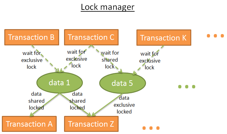
The lock manager is the process that gives and releases locks. Internally, it stores the locks in a hash table (where the key is the data to lock) and knows for each data:

• which transactions are locking the data
• which transactions are waiting for the data

Deadlock

But the use of locks can lead to a situation where 2 transactions are waiting forever for a data:

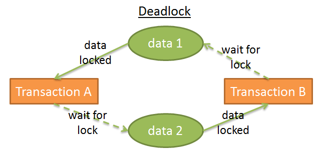
In this figure:

• transaction A has an exclusive lock on data1 and is waiting to get data2
• transaction B has an exclusive lock on data2 and is waiting to get data1

This is called a deadlock.

During a deadlock, the lock manager chooses which transaction to cancel (rollback) in order to remove the deadlock. This decision is not easy:

• Is it better to kill the transaction that modified the least amount of data (and therefore that will produce the least expensive rollback)?
• Is it better to kill the least aged transaction because the user of the other transaction has waited longer?
• Is it better to kill the transaction that will take less time to finish (and avoid a possible starvation)?
• In case of rollback, how many transactions will be impacted by this rollback?

But before making this choice, it needs to check if there are deadlocks.

The hash table can be seen as a graph (like in the previous figures). There is a deadlock if there is a cycle in the graph. Since it’s expensive to check for cycles (because the graph with all the locks is quite big), a simpler approach is often used: using a timeout. If a lock is not given within this timeout, the transaction enters a deadlock state.

The lock manager can also check before giving a lock if this lock will create a deadlock. But again it’s computationally expensive to do it perfectly. Therefore, these pre-checks are often a set of basic rules.

Two-phase locking

The simplest way to ensure a pure isolation is if a lock is acquired at the beginning of the transaction and released at the end of the transaction. This means that a transaction has to wait for all its locks before it starts and the locks held by a transaction are released when the transaction ends. It works but it produces a lot of time wasted to wait for all locks.

A faster way is the Two-Phase Locking Protocol (used by DB2 and SQL Server) where a transaction is divided into 2 phases:

• the growing phase where a transaction can obtain locks, but can’t release any lock.
• the shrinking phase where a transaction can release locks (on the data it has already processed and won’t process again), but can’t obtain new locks.

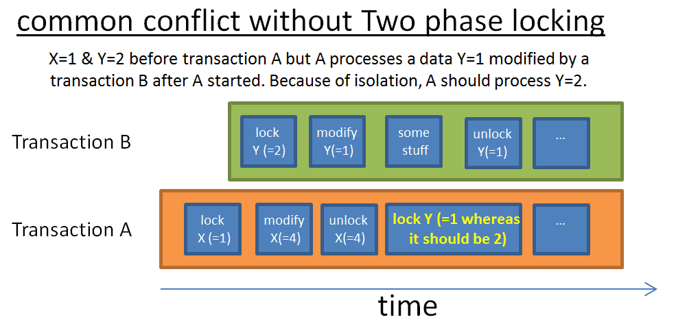
The idea behind these 2 simple rules is:

• to release the locks that aren’t used anymore to reduce the wait time of other transactions waiting for these locks
• to prevent from cases where a transaction gets data modified after the transaction started and therefore aren’t coherent with the first data the transaction acquired.

This protocol works well except if a transaction that modified a data and released the associated lock is cancelled (rolled back). You could end up in a case where another transaction reads the modified value whereas this value is going to be rolled back. To avoid this problem, all the exclusive locks must be released at the end of the transaction.

A few words

Of course a real database uses a more sophisticated system involving more types of locks (like intention locks) and more granularities (locks on a row, on a page, on a partition, on a table, on a tablespace) but the idea remains the same.

I only presented the pure lock-based approach. Data versioning is another way to deal with this problem.

The idea behind versioning is that:

• every transaction can modify the same data at the same time
• each transaction has its own copy (or version) of the data
• if 2 transactions modify the same data, only one modification will be accepted, the other will be refused and the associated transaction will be rolled back (and maybe re-run).

It increases the performance since:

• reader transactions don’t block writer transactions
• writer transactions don’t block reader transactions
• there is no overhead from the “fat and slow” lock manager

Everything is better than locks except when 2 transactions write the same data. Moreover, you can quickly end up with a huge disk space overhead.

Data versioning and locking are two different visions: optimistic locking vs pessimistic locking. They both have pros and cons; it really depends on the use case (more reads vs more writes). For a presentation on data versioning, I recommend this very good presentation on how PostgreSQL implements multiversion concurrency control.

Some databases like DB2 (until DB2 9.7) and SQL Server (except for snapshot isolation) are only using locks. Other like PostgreSQL, MySQL and Oracle use a mixed approach involving locks and data versioning. I’m not aware of a database using only data versioning (if you know a database based on a pure data versioning, feel free to tell me).

[UPDATE 08/20/2015] I was told by a reader that:

Firebird and Interbase use versioning without record locking.

Versioning has an interesting effect on indexes: sometimes a unique index contains duplicates, the index can have more entries than the table has rows, etc.

If you read the part on the different levels of isolation, when you increase the isolation level you increase the number of locks and therefore the time wasted by transactions to wait for their locks. This is why most databases don’t use the highest isolation level (Serializable) by default.

As always, you can check by yourself in the documentation of the main databases (for example MySQL , PostgreSQL or Oracle ).

Log manager

We’ve already seen that to increase its performances, a database stores data in memory buffers. But if the server crashes when the transaction is being committed, you’ll lose the data still in memory during the crash, which breaks the Durability of a transaction.

You can write everything on disk but if the server crashes, you’ll end up with the data half written on disk, which breaks the Atomicity of a transaction.

Any modification written by a transaction must be undone or finished.

To deal with this problem, there are 2 ways:

• Shadow copies/pages: Each transaction creates its own copy of the database (or just a part of the database) and works on this copy. In case of error, the copy is removed. In case of success, the database switches instantly the data from the copy with a filesystem trick then it removes the “old” data.
• Transaction log: A transaction log is a storage space. Before each write on disk, the database writes an info on the transaction log so that in case of crash/cancel of a transaction, the database knows how to remove (or finish) the unfinished transaction.

WAL

The shadow copies/pages creates a huge disk overhead when used on large databases involving many transactions. That’s why modern databases use a transaction log. The transaction log must be stored on a stable storage. I won’t go deeper on storage technologies but using (at least) RAID disks is mandatory to prevent from a disk failure.

Most databases (at least Oracle, SQL Server , DB2 , PostgreSQL , MySQL and SQLite ) deal with the transaction log using the Write-Ahead Logging protocol (WAL). The WAL protocol is a set of 3 rules:

• 1. Each modification into the database produces a log record, and the log record must be written into the transaction log before the data is written on disk.
• 2. The log records must be written in order; a log record A that happens before a log record B must but written before B
• 3. When a transaction is committed, the commit order must be written on the transaction log before the transaction ends up successfully.

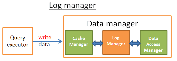
This job is done by a log manager. An easy way to see it is that between the cache manager and the data access manager (that writes data on disk) the log manager writes every update/delete/create/commit/rollback on the transaction log before they’re written on disk. Easy, right?

WRONG ANSWER! After all we’ve been through, you should know that everything related to a database is cursed by the “database effect”. More seriously, the problem is to find a way to write logs while keeping good performances. If the writes on the transaction log are too slow they will slow down everything.

ARIES

In 1992, IBM researchers “invented” an enhanced version of WAL called ARIES. ARIES is more or less used by most modern databases. The logic might not be the same but the concepts behind ARIES are used everywhere. I put the quotes on invented because, according to this MIT course , the IBM researchers did “nothing more than writing the good practices of transaction recovery”. Since I was 5 when the ARIES paper was published, I don’t care about this old gossip from bitter researchers. In fact, I only put this info to give you a break before we start this last technical part. I’ve read a huge part of the research paper on ARIES and I find it very interesting! In this part I’ll only give you an overview of ARIES but I strongly recommend to read the paper if you want a real knowledge.

ARIES stands for Algorithms for Recovery and Isolation Exploiting Semantics.

The aim of this technique is double:

• 1. Having good performances when writing logs
• 2. Having a fast and reliable recovery

There are multiple reasons a database has to rollback a transaction:

• Because the user cancelled it
• Because of server or network failures
• Because the transaction has broken the integrity of the database (for example you have a UNIQUE constraint on a column and the transaction adds a duplicate)
• Because of deadlocks

Sometimes (for example, in case of network failure), the database can recover the transaction.

How is that possible? To answer this question, we need to understand the information stored in a log record.

The logs

Each operation (add/remove/modify) during a transaction produces a log. This log record is composed of:

• LSN: A unique Log Sequence Number. This LSN is given in a chronological order*. This means that if an operation A happened before an operation B the LSN of log A will be lower than the LSN of log B.
• TransID: the id of the transaction that produced the operation.
• PageID: the location on disk of the modified data. The minimum amount of data on disk is a page so the location of the data is the location of the page that contains the data.
• PrevLSN: A link to the previous log record produced by the same transaction.
• UNDO: a way to remove the effect of the operation

For example, if the operation is an update, the UNDO will store either the value/state of the updated element before the update (physical UNDO) or the reverse operation to go back at the previous state (logical UNDO)**.

• REDO: a way replay the operation

Likewise, there are 2 ways to do that. Either you store the value/state of the element after the operation or the operation itself to replay it.

• …: (FYI, an ARIES log has 2 others fields: the UndoNxtLSN and the Type).

Moreover, each page on disk (that stores the data, not the log) has id of the log record (LSN) of the last operation that modified the data.

The way the LSN is given is more complicated because it is linked to the way the logs are stored. But the idea remains the same.

ARIES uses only logical UNDO because it’s a real mess to deal with physical UNDO.

Note: From my little knowledge, only PostgreSQL is not using an UNDO. It uses instead a garbage collector daemon that removes the old versions of data. This is linked to the implementation of the data versioning in PostgreSQL.

To give you a better idea, here is a visual and simplified example of the log records produced by the query “UPDATE FROM PERSON SET AGE = 18;”. Let’s say this query is executed in transaction 18.

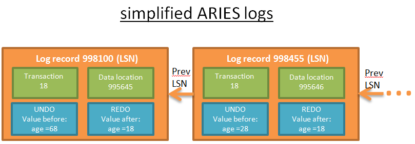
Each log has a unique LSN. The logs that are linked belong to the same transaction. The logs are linked in a chronological order (the last log of the linked list is the log of the last operation).

To conclude

Before writing this article, I knew how big the subject was and I knew it would take time to write an in-depth article about it. It turned out that I was very optimistic and I spent twice more time than expected, but I learned a lot.

If you want a good overview about databases, I recommend reading the research paper “Architecture of a Database System “. This is a good introduction on databases (110 pages) and for once it’s readable by non-CS guys. This paper helped me a lot to find a plan for this article and it’s not focused on data structures and algorithms like my article but more on the architecture concepts.

If you read this article carefully you should now understand how powerful a database is. Since it was a very long article, let me remind you about what we’ve seen:

• an overview of the B+Tree indexes
• a global overview of a database
• an overview of the cost based optimization with a strong focus on join operators
• an overview of the buffer pool management
• an overview of the transaction management

But a database contains even more cleverness. For example, I didn’t speak about some touchy problems like:

• how to manage clustered databases and global transactions
• how to take a snapshot when the database is still running
• how to efficiently store (and compress) data
• how to manage memory

So, think twice when you have to choose between a buggy NoSQL database and a rock-solid relational database. Don’t get me wrong, some NoSQL databases are great. But they’re still young and answering specific problems that concern a few applications.

To conclude, if someone asks you how a database works, instead of running away you’ll now be able to answer:

Otherwise you can give him/her this article.